9  WagePredictors

9.1 Introduction

This analysis examines whether demographic characteristics, age, marital status, employment, and health variables can predict whether someone earns a comparatively higher or lower wage. A binary wage outcome was created based on the median wage. Classical statistical tests (t-tests, ANOVA, and chi-square) and a logistic regression model were used to identify meaningful predictors of income category.

Note

This chapter demonstrates combining classical hypothesis testing with predictive modeling (logistic regression) to examine wage differences.

9.2 Data Preparation

data("Wage")

wage_median <- median(Wage$wage, na.rm = TRUE)

Wage <- Wage %>%
  mutate(
    WageCategory = case_when(
      wage > wage_median ~ "High",
      wage < wage_median ~ "Low",
      TRUE ~ NA_character_
    )
  ) %>%
  filter(!is.na(WageCategory))

Wage$WageCategory <- factor(Wage$WageCategory, levels = c("Low", "High"))

table(Wage$WageCategory) %>%
  as.data.frame() %>%
  knitr::kable() %>%
  kableExtra::kable_styling(full_width = FALSE)

Table 9.1: Number of observations classified as low versus high wage earners.

Var1	Freq
Low	1447
High	1483

9.3 Cleaning Factor Variables

clean_factor <- function(x) {
  x <- as.character(x)
  x <- str_replace(x, "^[0-9]+\\.\\s*", "")
  factor(x)
}

Wage <- Wage %>%
  mutate(
    race       = clean_factor(race),
    education  = clean_factor(education),
    jobclass   = clean_factor(jobclass),
    health     = clean_factor(health),
    health_ins = clean_factor(health_ins),
    maritl     = clean_factor(maritl)
  )

9.4 Age Differences (T-Test)

Wage %>%
  group_by(WageCategory) %>%
  summarise(
    mean_age = mean(age, na.rm = TRUE),
    sd_age   = sd(age, na.rm = TRUE),
    n        = n()
  ) %>%
  knitr::kable(digits = 2) %>%
  kableExtra::kable_styling(full_width = FALSE)

Table 9.2: Mean age and standard deviation by wage category.

WageCategory	mean_age	sd_age	n
Low	40.01	12.67	1447
High	44.69	9.82	1483

age_ttest <- t.test(age ~ WageCategory, data = Wage)
age_ttest

    Welch Two Sample t-test

data:  age by WageCategory
t = -11.143, df = 2724.7, p-value < 2.2e-16
alternative hypothesis: true difference in means between group Low and group High is not equal to 0
95 percent confidence interval:
 -5.496555 -3.851525
sample estimates:
 mean in group Low mean in group High 
          40.01106           44.68510 

9.5 Interpretation

A Welch two-sample t-test showed a significant difference in age between high and low wage earners, t(2724.7) = −11.14, p < .001. High earners were, on average, older than low earners, indicating a positive association between age and wage.

9.6 Education and Wage (Anova)

wage_edu_aov <- aov(wage ~ education, data = Wage)

summary(wage_edu_aov)[[1]] %>%
  as.data.frame() %>%
  knitr::kable(digits = 2) %>%
  kableExtra::kable_styling(full_width = FALSE)

Table 9.3: ANOVA table examining the effect of education on wage.

	Df	Sum Sq	Mean Sq	F value	Pr(>F)
education	4	1242703	310675.73	228.55	0
Residuals	2925	3976086	1359.35	NA	NA

9.7 Interpretation

The ANOVA showed a significant effect of education on wage, F(4, 2925) = 228.5, p < .001. Wages increased consistently with higher levels of education, suggesting that education is a strong predictor of income.

9.8 Marital Status and Wage (Chi-Square)

wage_maritl_table <- table(Wage$WageCategory, Wage$maritl)

wage_maritl_table %>%
  as.data.frame.matrix() %>%
  knitr::kable() %>%
  kableExtra::kable_styling(full_width = FALSE)

Table 9.4: Contingency table of wage category by marital status.

	Divorced	Married	Never Married	Separated	Widowed
Low	114	817	470	37	9
High	86	1202	169	18	8

chisq_wage_maritl <- chisq.test(wage_maritl_table)
chisq_wage_maritl

    Pearson's Chi-squared test

data:  wage_maritl_table
X-squared = 225.33, df = 4, p-value < 2.2e-16

cramer_v <- CramerV(wage_maritl_table)
cramer_v

[1] 0.2773195

9.9 Interpretation

The chi-square test showed a significant association between wage category and marital status, χ²(4) = 225.33, p < .001. Cramer’s V = 0.277 indicates a moderate association. Married individuals were more represented in the high-wage group, while never-married individuals were more represented in the low-wage group.

9.10 Train Test Split

set.seed(123)
split_flag <- sample.split(Wage$WageCategory, SplitRatio = 0.7)

train_data <- subset(Wage, split_flag == TRUE)
test_data  <- subset(Wage, split_flag == FALSE)

9.11 Logistic Regression Model

logit_model <- glm(
  WageCategory ~ age + education + jobclass + maritl + health + health_ins,
  data = train_data,
  family = binomial
)

summary(logit_model)

Call:
glm(formula = WageCategory ~ age + education + jobclass + maritl + 
    health + health_ins, family = binomial, data = train_data)

Coefficients:
                          Estimate Std. Error z value Pr(>|z|)    
(Intercept)              -3.906039   0.410689  -9.511  < 2e-16 ***
age                       0.016967   0.005301   3.201  0.00137 ** 
educationAdvanced Degree  2.878189   0.272729  10.553  < 2e-16 ***
educationCollege Grad     2.356742   0.243963   9.660  < 2e-16 ***
educationHS Grad          0.654597   0.231391   2.829  0.00467 ** 
educationSome College     1.399887   0.238876   5.860 4.62e-09 ***
jobclassInformation       0.128700   0.110463   1.165  0.24398    
maritlMarried             0.816820   0.209849   3.892 9.92e-05 ***
maritlNever Married      -0.480261   0.245800  -1.954  0.05072 .  
maritlSeparated          -0.213755   0.474737  -0.450  0.65252    
maritlWidowed             0.191127   0.599294   0.319  0.74979    
health>=Very Good         0.325054   0.121269   2.680  0.00735 ** 
health_insYes             1.372473   0.123232  11.137  < 2e-16 ***
---
Signif. codes:  0 '***' 0.001 '**' 0.01 '*' 0.05 '.' 0.1 ' ' 1

(Dispersion parameter for binomial family taken to be 1)

    Null deviance: 2843.0  on 2050  degrees of freedom
Residual deviance: 2115.4  on 2038  degrees of freedom
AIC: 2141.4

Number of Fisher Scoring iterations: 4

odds_ratios <- exp(coef(logit_model))
odds_ratios

             (Intercept)                      age educationAdvanced Degree 
              0.02012005               1.01711169              17.78204218 
   educationCollege Grad         educationHS Grad    educationSome College 
             10.55650582               1.92436665               4.05474320 
     jobclassInformation            maritlMarried      maritlNever Married 
              1.13734877               2.26329134               0.61862205 
         maritlSeparated            maritlWidowed        health>=Very Good 
              0.80754605               1.21061266               1.38410575 
           health_insYes 
              3.94509346 

9.12 Generate Predictions

test_probs <- predict(logit_model, newdata = test_data, type = "response")

test_pred_class <- ifelse(test_probs > 0.5, "High", "Low")
test_pred_class <- factor(test_pred_class, levels = c("Low", "High"))

conf_mat <- caret::confusionMatrix(
  data      = test_pred_class,
  reference = test_data$WageCategory,
  positive  = "High"
)

9.13 Model Performance

conf_mat$table %>%
  as.data.frame.matrix() %>%
  knitr::kable() %>%
  kableExtra::kable_styling(full_width = FALSE)

Table 9.5: Confusion matrix for predicting high vs low wage.

	Low	High
Low	304	119
High	130	326

9.14 Checking for Accuracy

conf_mat$overall %>%
  as.data.frame() %>%
  knitr::kable(digits = 3) %>%
  kableExtra::kable_styling(full_width = FALSE)

Table 9.6: Overall performance statistics for the logistic regression model.

	.
Accuracy	0.717
Kappa	0.433
AccuracyLower	0.686
AccuracyUpper	0.746
AccuracyNull	0.506
AccuracyPValue	0.000
McnemarPValue	0.526

roc_obj <- roc(
  response = test_data$WageCategory,
  predictor = test_probs,
  levels = c("Low", "High")
)

Setting direction: controls < cases

plot(roc_obj, main = "ROC Curve for WageCategory Model")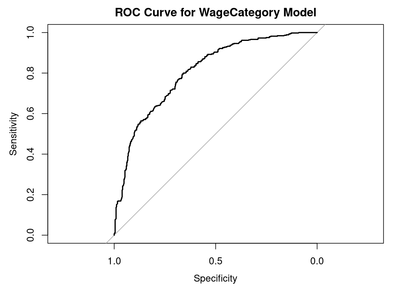

Figure 9.1: ROC Curve for High vs Low Wage Classification.

auc_value <- auc(roc_obj)
auc_value

Area under the curve: 0.8063

9.15 Conclusion

This analysis showed that high earners were older on average, and education had one of the strongest effects on wage. Income increased consistently with higher education levels. Married workers were more likely to be high earners, while never-married individuals were more often in the low-wage group.

The logistic regression model confirmed these patterns. Education emerged as the strongest predictor of high wage status. Age, marital status, health, and health insurance also contributed positively to the likelihood of earning a higher wage. The model achieved approximately 71.7% accuracy on the test set, indicating solid predictive performance.

Future analyses could incorporate additional life-course variables such as childhood socioeconomic status or family background to better understand long-term influences on adult income.