7  FloridaCrime

7.1 Introduction

This chapter analyzes data from Florida counties to examine which factors—income, education, and urban environment—best predict county-level crime rates. Using descriptive statistics, visualizations, correlations, and regression models, I evaluate whether urban population, income, and high school graduation rates are associated with crime.

Note

This analysis focuses on relationships (correlations and regression). These results can suggest patterns, but they do not prove causation.

7.2 Data Import and Cleaning

data <- read_excel("FloridaCountyCrimeRates.xlsx")

data <- data %>%
  rename(
    County = County,
    Crime = C,
    Income = I,
    HighSchoolGrad = HS,
    UrbanPop = U
  )

data$County <- str_to_title(tolower(data$County))

head(data) %>%
  knitr::kable() %>%
  kableExtra::kable_styling(full_width = FALSE)

Table 7.1: Preview of the Florida county dataset.

County	Crime	Income	HighSchoolGrad	UrbanPop
Alachua	104	22.1	82.7	73.2
Baker	20	25.8	64.1	21.5
Bay	64	24.7	74.7	85.0
Bradford	50	24.6	65.0	23.2
Brevard	64	30.5	82.3	91.9
Broward	94	30.6	76.8	98.9

7.3 Descriptive Statistics

psych::describe(data[, c("Crime", "Income", "HighSchoolGrad", "UrbanPop")]) %>%
  as.data.frame() %>%
  tibble::rownames_to_column(var = "Variable") %>%
  knitr::kable(digits = 2) %>%
  kableExtra::kable_styling(full_width = FALSE)

Table 7.2: Descriptive statistics for Crime, Income, High School Graduation, and Urban Population.

Variable	vars	n	mean	sd	median	trimmed	mad	min	max	range	skew	kurtosis	se
Crime	1	67	52.40	28.19	52.0	51.60	25.20	0.0	128.0	128.0	0.32	-0.29	3.44
Income	2	67	24.51	4.68	24.6	24.33	5.34	15.4	35.6	20.2	0.34	-0.70	0.57
HighSchoolGrad	3	67	69.49	8.86	69.0	69.48	11.56	54.5	84.9	30.4	-0.02	-1.30	1.08
UrbanPop	4	67	49.56	33.97	44.6	49.75	42.40	0.0	99.6	99.6	-0.02	-1.49	4.15

7.4 Visualization

ggplot(data, aes(x = Income, y = Crime)) +
  geom_point() +
  geom_smooth(method = "lm", se = TRUE) +
  theme_minimal() +
  labs(
    title = "Income vs Crime (Florida Counties)",
    x = "Income",
    y = "Crime"
  )

`geom_smooth()` using formula = 'y ~ x'

Figure 7.1: Scatterplot of Income versus Crime with a fitted regression line. This evaluates whether counties with higher income tend to have higher or lower crime rates.

ggplot(data, aes(x = Crime)) +
  geom_histogram(bins = 20, fill = "skyblue", color = "white") +
  theme_minimal() +
  labs(
    title = "Distribution of Crime Rates (Florida Counties)",
    x = "Crime",
    y = "Number of Counties"
  )

Figure 7.2: Histogram of county-level crime rates in Florida.

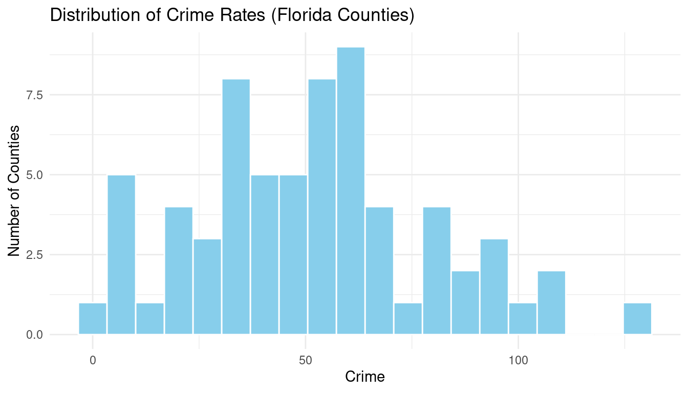
The scatterplot suggests a positive relationship between income and crime, meaning counties with higher income may also show somewhat higher crime rates. The histogram indicates that most counties cluster around moderate crime rates, with a smaller number of counties showing higher levels.

Tip

A positive relationship between income and crime can occur if higher-income counties are also more urban. Urbanization can act as a confounding variable, which is why multiple regression is useful.

7.5 Correlation Matrix

cor_matrix <- cor(
  data[, c("Crime", "Income", "HighSchoolGrad", "UrbanPop")],
  use = "pairwise.complete.obs"
)

ggcorrplot::ggcorrplot(cor_matrix, lab = TRUE, title = "Correlation Matrix")

Warning: `aes_string()` was deprecated in ggplot2 3.0.0.
ℹ Please use tidy evaluation idioms with `aes()`.
ℹ See also `vignette("ggplot2-in-packages")` for more information.
ℹ The deprecated feature was likely used in the ggcorrplot package.
  Please report the issue at <https://github.com/kassambara/ggcorrplot/issues>.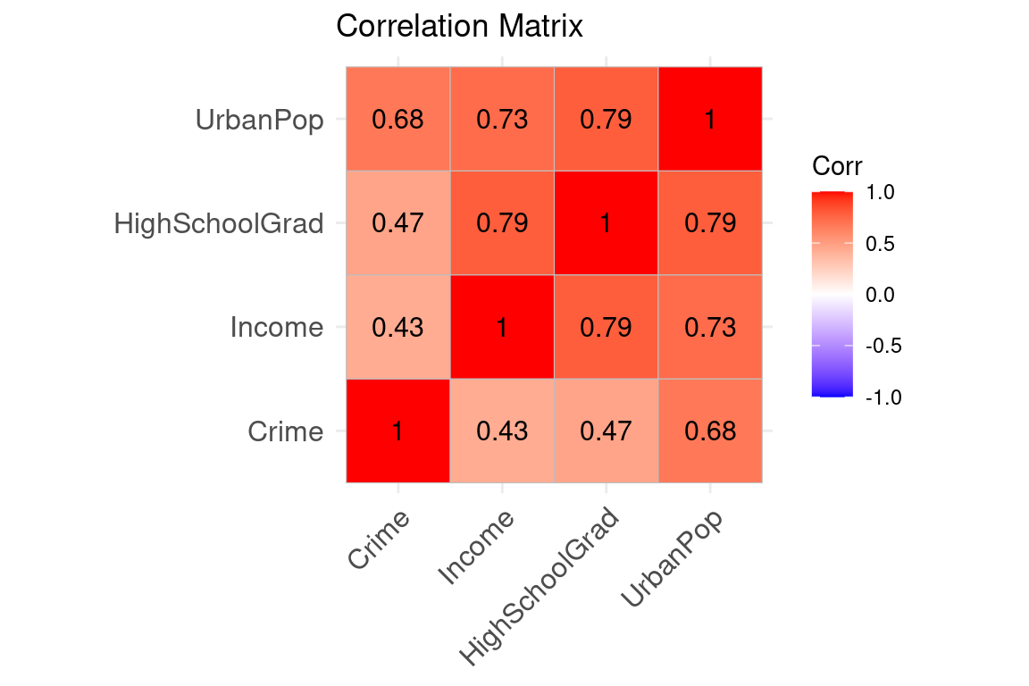

Figure 7.3: Correlation matrix for Crime, Income, High School Graduation, and Urban Population.

7.6 Regression Models

broom::tidy(m1) %>%
  knitr::kable(digits = 3) %>%
  kableExtra::kable_styling(full_width = FALSE)

Table 7.3: Regression model predicting Crime from Income.

term	estimate	std.error	statistic	p.value
(Intercept)	-11.606	16.786	-0.691	0.492
Income	2.611	0.673	3.881	0.000

broom::tidy(m2) %>%
  knitr::kable(digits = 3) %>%
  kableExtra::kable_styling(full_width = FALSE)

Table 7.4: Multiple regression predicting Crime from Income, High School Graduation, and Urban Population.

term	estimate	std.error	statistic	p.value
(Intercept)	59.715	28.590	2.089	0.041
Income	-0.383	0.941	-0.407	0.685
HighSchoolGrad	-0.467	0.554	-0.843	0.403
UrbanPop	0.697	0.129	5.399	0.000

bind_rows(
  broom::glance(m1) %>% mutate(Model = "Income only"),
  broom::glance(m2) %>% mutate(Model = "Multiple regression")
) %>%
  select(Model, r.squared, adj.r.squared, AIC, BIC, sigma) %>%
  knitr::kable(digits = 3) %>%
  kableExtra::kable_styling(full_width = FALSE)

Table 7.5: Model fit statistics for the two regression models.

Model	r.squared	adj.r.squared	AIC	BIC	sigma
Income only	0.188	0.176	628.605	635.219	25.598
Multiple regression	0.473	0.448	603.676	614.700	20.953

AIC(m1, m2) %>%
  as.data.frame() %>%
  tibble::rownames_to_column(var = "Model") %>%
  knitr::kable(digits = 2) %>%
  kableExtra::kable_styling(full_width = FALSE)

Table 7.6: AIC comparison of the simple (Income only) vs. multiple regression model.

Model	df	AIC
m1	3	628.60
m2	5	603.68

7.7 Conclusion

The correlation matrix suggests crime is most strongly associated with urban population. Income and high school graduation also show associations with crime, but these relationships should be interpreted cautiously because they may reflect differences between urban and rural counties. In the multiple regression model, urban population remains the strongest predictor after accounting for income and education.

7.8 Memo to the Chief of the Florida Police Department

Based on this analysis, the multiple regression model provides the best prediction of Florida’s county-level crime rates. The results suggest that urbanization is the strongest and most consistent predictor of crime, meaning that counties with larger urban populations tend to experience higher crime rates. To reduce crime statewide, the Florida Police Department should prioritize resources and targeted interventions in highly urbanized counties.

Before implementing solutions, it would be valuable to identify which types of crimes are most common in high-crime urban areas. If crime is primarily driven by theft, vandalism, or assault, increasing patrol coverage and visible deterrence may help. However, if a substantial portion is linked to substance use, domestic violence, or mental health crises, then expanding partnerships with social services—such as mental health professionals and social workers—may be equally important. A balanced approach combining enforcement with prevention and community support is likely to be most effective in reducing crime in Florida’s urban counties.