5  Sleep_and_Exercise_Analysis

5.1 Introduction

This chapter analyzes a dataset examining whether different exercise routines are associated with improvements in sleep. Using data cleaning, merging, descriptive statistics, visualizations, t-tests, and one-way ANOVA with post-hoc comparisons, I evaluate changes in sleep duration (post–pre) and sleep efficiency across exercise groups.

Note

This analysis demonstrates a complete reproducible workflow, including importing messy real-world data, cleaning variables, visualizing patterns, and performing statistical inference.

file_path <- "midterm_sleep_exercise.xlsx"

# (Optional) quick check during development:
# readxl::excel_sheets(file_path)

participant_info <- readxl::read_xlsx(
  file_path,
  sheet = "participant_info_midterm"
)

sleep_data <- readxl::read_xlsx(
  file_path,
  sheet = "sleep_data_midterm"
)

participant_info <- janitor::clean_names(participant_info)
sleep_data       <- janitor::clean_names(sleep_data)

5.2 Data Cleaning and Preparation

merged_data <- left_join(participant_info, sleep_data, by = "id") %>%
  mutate(
    sex = case_when(
      tolower(sex) %in% c("female","fem","f","femalee") ~ "Female",
      tolower(sex) %in% c("male","mal","m","malee") ~ "Male",
      TRUE ~ NA_character_
    ),
    exercise_group = case_when(
      str_detect(tolower(exercise_group), "c\\+w|cw") ~ "C+W",
      str_detect(tolower(exercise_group), "cardio") ~ "Cardio",
      str_detect(tolower(exercise_group), "weights|weight") ~ "Weights",
      str_detect(tolower(exercise_group), "none") ~ "None",
      TRUE ~ exercise_group
    ),
    age = as.numeric(age),
    pre_sleep = as.numeric(str_extract(pre_sleep, "\\d+\\.\\d+")),
    post_sleep = as.numeric(post_sleep),
    sleep_difference = post_sleep - pre_sleep,
    agegroup2 = case_when(
      age < 40 ~ "<40",
      age >= 40 ~ ">=40",
      TRUE ~ NA_character_
    )
  ) %>%
  filter(!is.na(sleep_difference))

list(
  exercise_group = table(merged_data$exercise_group),
  sex = table(merged_data$sex),
  agegroup2 = table(merged_data$agegroup2)
) %>%
  knitr::kable()

Table 5.1: Number of participants by exercise group, sex, and age group.

Var1 Freq C+W 3 Cardio 34 N 2 None 15 Weights 19

Var1 Freq Female 40 Male 33

Var1 Freq <40 57 >=40 16

5.3 Descriptive Statistics

overall_summary <- merged_data %>%
  summarise(
    mean_sleep_diff = mean(sleep_difference),
    sd_sleep_diff = sd(sleep_difference),
    min_sleep_diff = min(sleep_difference),
    max_sleep_diff = max(sleep_difference),
    mean_sleep_eff = mean(sleep_efficiency),
    sd_sleep_eff = sd(sleep_efficiency),
    min_sleep_eff = min(sleep_efficiency),
    max_sleep_eff = max(sleep_efficiency)
  )

knitr::kable(overall_summary, digits = 2)

Table 5.2: Overall descriptive statistics for sleep improvement and sleep efficiency.

mean_sleep_diff	sd_sleep_diff	min_sleep_diff	max_sleep_diff	mean_sleep_eff	sd_sleep_eff	min_sleep_eff	max_sleep_eff
0.68	0.63	-1.1	2	84.16	5.98	71.7	101.5

group_summary <- merged_data %>%
  group_by(exercise_group) %>%
  summarise(
    mean_sleep_diff = mean(sleep_difference),
    sd_sleep_diff = sd(sleep_difference),
    mean_sleep_eff = mean(sleep_efficiency),
    sd_sleep_eff = sd(sleep_efficiency),
    n = n()
  )

knitr::kable(group_summary, digits = 2)

Table 5.3: Descriptive statistics for sleep improvement and sleep efficiency by exercise group.

exercise_group	mean_sleep_diff	sd_sleep_diff	mean_sleep_eff	sd_sleep_eff	n
C+W	1.10	0.10	90.23	3.76	3
Cardio	0.97	0.44	86.56	5.94	34
N	0.30	0.85	81.30	0.28	2
None	0.09	0.64	81.37	6.10	15
Weights	0.61	0.60	81.43	3.92	19

5.4 Visualization of Sleep Outcomes

ggplot(merged_data, aes(x = exercise_group, y = sleep_difference, fill = exercise_group)) +
  geom_boxplot() +
  labs(
    title = "Sleep Improvement by Exercise Group",
    x = "Exercise Group",
    y = "Sleep Difference (Post - Pre)"
  ) +
  theme_minimal() +
  theme(legend.position = "none")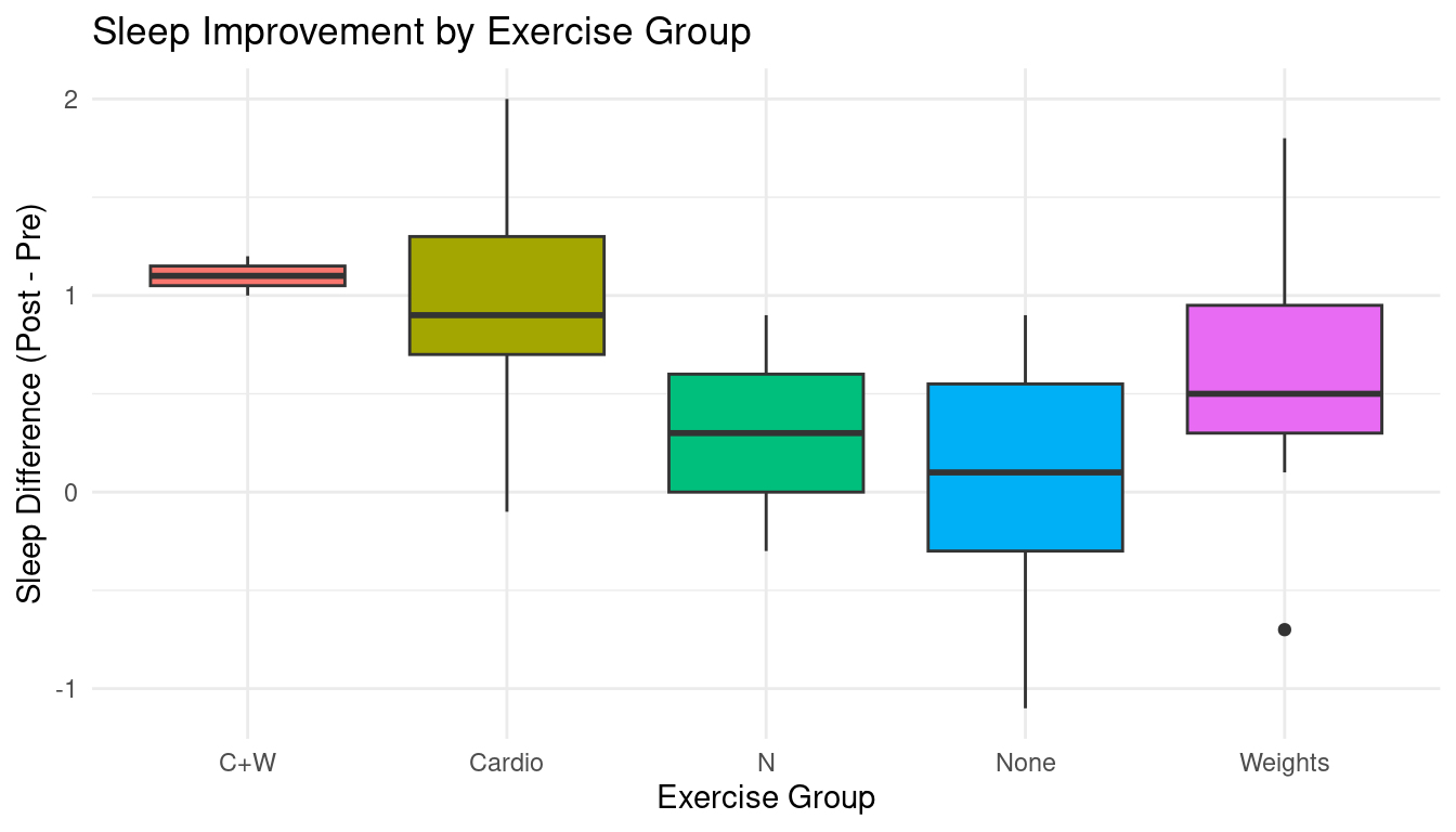

Figure 5.1: Boxplots of sleep improvement across exercise groups.

ggplot(merged_data, aes(x = exercise_group, y = sleep_efficiency, fill = exercise_group)) +
  geom_boxplot() +
  labs(
    title = "Sleep Efficiency by Exercise Group",
    x = "Exercise Group",
    y = "Sleep Efficiency (%)"
  ) +
  theme_minimal() +
  theme(legend.position = "none")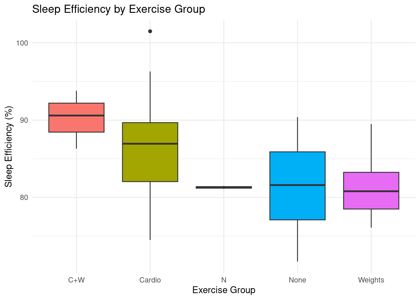

Figure 5.2: Sleep efficiency by exercise group.

ggplot(merged_data, aes(x = sleep_difference, y = sleep_efficiency)) +
  geom_point(color = "blue") +
  geom_smooth(method = "lm", se = FALSE, color = "red") +
  labs(
    title = "Sleep Improvement vs Sleep Efficiency",
    x = "Sleep Difference",
    y = "Sleep Efficiency (%)"
  ) +
  theme_minimal()

`geom_smooth()` using formula = 'y ~ x'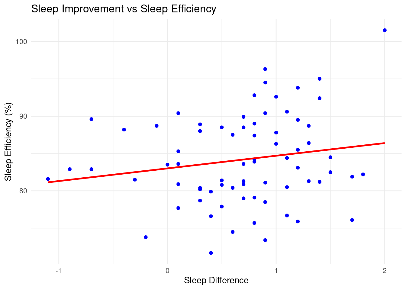

Figure 5.3: Relationship between sleep improvement and sleep efficiency.

5.5 Independent Sample T-Test

t_sex <- t.test(
  sleep_difference ~ sex,
  data = merged_data %>% filter(!is.na(sex))
)

t_sex

    Welch Two Sample t-test

data:  sleep_difference by sex
t = 1.3852, df = 64.335, p-value = 0.1708
alternative hypothesis: true difference in means between group Female and group Male is not equal to 0
95 percent confidence interval:
 -0.09075179  0.50135785
sample estimates:
mean in group Female   mean in group Male 
            0.775000             0.569697 

t_age <- t.test(
  sleep_difference ~ agegroup2,
  data = merged_data %>% filter(!is.na(agegroup2))
)

t_age

    Welch Two Sample t-test

data:  sleep_difference by agegroup2
t = -1.357, df = 40.85, p-value = 0.1822
alternative hypothesis: true difference in means between group <40 and group >=40 is not equal to 0
95 percent confidence interval:
 -0.45511702  0.08932755
sample estimates:
 mean in group <40 mean in group >=40 
         0.6421053          0.8250000 

Tip

Neither sex nor age group showed statistically significant differences in sleep improvement, suggesting exercise effects are consistent across demographic groups.

5.6 One-way ANOVA and Post-hoc Comparisons

anova_sleep_diff <- aov(
  sleep_difference ~ exercise_group,
  data = merged_data
)

summary(anova_sleep_diff)

               Df Sum Sq Mean Sq F value   Pr(>F)    
exercise_group  4  9.061  2.2653    8.02 2.34e-05 ***
Residuals      68 19.206  0.2824                     
---
Signif. codes:  0 '***' 0.001 '**' 0.01 '*' 0.05 '.' 0.1 ' ' 1

eta_squared(anova_sleep_diff)

For one-way between subjects designs, partial eta squared is equivalent
  to eta squared. Returning eta squared.

# Effect Size for ANOVA

Parameter      | Eta2 |       95% CI
------------------------------------
exercise_group | 0.32 | [0.15, 1.00]

- One-sided CIs: upper bound fixed at [1.00].

TukeyHSD(anova_sleep_diff)

  Tukey multiple comparisons of means
    95% family-wise confidence level

Fit: aov(formula = sleep_difference ~ exercise_group, data = merged_data)

$exercise_group
                     diff          lwr         upr     p adj
Cardio-C+W     -0.1294118 -1.026386819  0.76756329 0.9942482
N-C+W          -0.8000000 -2.159530534  0.55953053 0.4720308
None-C+W       -1.0133333 -1.955243717 -0.07142295 0.0287638
Weights-C+W    -0.4894737 -1.414711770  0.43576440 0.5772427
N-Cardio       -0.6705882 -1.754206665  0.41303019 0.4203454
None-Cardio    -0.8839216 -1.345549991 -0.42229315 0.0000102
Weights-Cardio -0.3600619 -0.786642681  0.06651884 0.1375430
None-N         -0.2133333 -1.334430932  0.90776426 0.9835831
Weights-N       0.3105263 -0.796600673  1.41765330 0.9338316
Weights-None    0.5238596  0.009464793  1.03825451 0.0438730

anova_sleep_eff <- aov(
  sleep_efficiency ~ exercise_group,
  data = merged_data
)

summary(anova_sleep_eff)

               Df Sum Sq Mean Sq F value  Pr(>F)   
exercise_group  4  580.7   145.2   4.954 0.00145 **
Residuals      68 1992.4    29.3                   
---
Signif. codes:  0 '***' 0.001 '**' 0.01 '*' 0.05 '.' 0.1 ' ' 1

eta_squared(anova_sleep_eff)

For one-way between subjects designs, partial eta squared is equivalent
  to eta squared. Returning eta squared.

# Effect Size for ANOVA

Parameter      | Eta2 |       95% CI
------------------------------------
exercise_group | 0.23 | [0.07, 1.00]

- One-sided CIs: upper bound fixed at [1.00].

TukeyHSD(anova_sleep_eff)

  Tukey multiple comparisons of means
    95% family-wise confidence level

Fit: aov(formula = sleep_efficiency ~ exercise_group, data = merged_data)

$exercise_group
                      diff        lwr        upr     p adj
Cardio-C+W     -3.67745098 -12.813473  5.4585710 0.7912049
N-C+W          -8.93333333 -22.780654  4.9139870 0.3775963
None-C+W       -8.86666667 -18.460372  0.7270383 0.0835904
Weights-C+W    -8.80175439 -18.225646  0.6221370 0.0784124
N-Cardio       -5.25588235 -16.292936  5.7811713 0.6708789
None-Cardio    -5.18921569  -9.891072 -0.4873598 0.0232689
Weights-Cardio -5.12430341  -9.469186 -0.7794209 0.0127670
None-N          0.06666667 -11.352126 11.4854595 1.0000000
Weights-N       0.13157895 -11.144918 11.4080760 0.9999997
Weights-None    0.06491228  -5.174389  5.3042138 0.9999997

5.7 Interpretation and Recommendations

Important

Exercise significantly improves both sleep duration and sleep efficiency. Cardio and combined cardio and weight training show the strongest benefits, while no exercise produces the smallest improvements.

Cardio-based exercise routines produced the largest sleep improvements and efficiency gains. Individuals who did not exercise showed the smallest improvements. These findings suggest that cardio or combined cardio and strength training may be the most effective exercise strategies for improving sleep.

5.8 Reflection

This analysis strengthened my ability to work with messy datasets, perform statistical analysis, and interpret results. I also improved my understanding of reproducible workflows and visualization techniques. Moving forward, I aim to continue improving my coding efficiency and statistical interpretation skills.